Example Diagrams
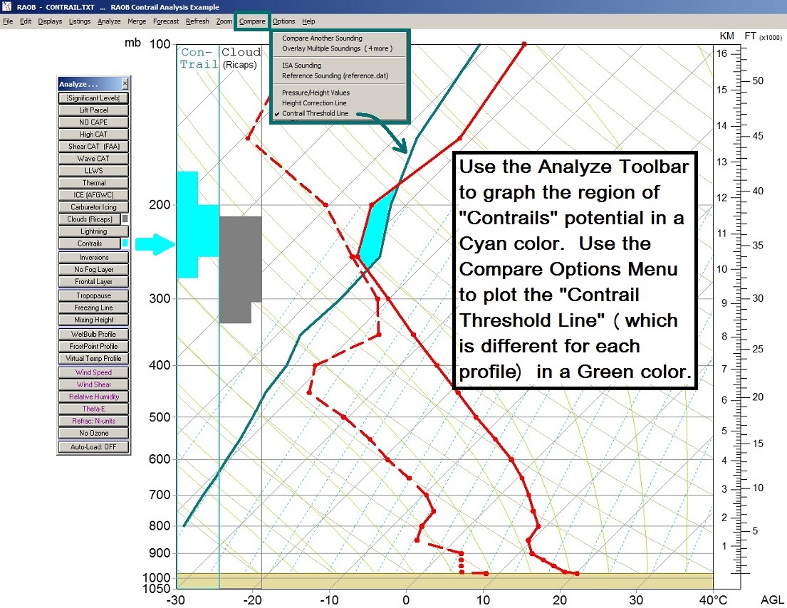
Example of the popular Skew-T diagram

Example of a Skew-T diagram.
Along the left side of the diagram are graphic analyses of CAT, LLWS (light), Thermal Turbulence, Icing (clear), Clouds (scattered), Lightning potential, Contrail potential. Key sounding alphanumeric parameters and indices are listed in upper-right section of the diagram, including Station Elevation, Significant Levels, SWEAT, CAPE data. To the right is a thermodynamically coupled height scale that separates the diagram from the wind plots. All displayed data is automatically updated when using the optional Interactive/Hodograph module.
Example of the flexible Emagram diagram

Example of an Emagram diagram
The Emagram is great for sounding plots reaching above 100 millibars. (Data can be plotted up to the 1 mb level.) It is also best for viewing lapse rate changes, especially as they relate to inversions (shown here as five graphical overlays). This example shows Subsidence and Radiation inversions. RAOB can also analyze and display frontal inversions (see next example). This example also has a mini-hodograph drawn in the upper-right corner of the emagram and the ICAO Standard Atmosphere is plotted as a black solid line. (Inversions can only plotted when the optional Analytic module is used.)
Example of a Frontal Layer plot

Example of a Frontal Layer plot
This Emagram displays two frontal inversions (light green) and a Warm front layer (rose color). RAOB analyzes frontal layers from the hodograph’s thermal wind data. (Frontal analyses are only available with the Fronts & Forecast module.) This example also has a mini-hodograph drawn in the upper-right corner of the emagram. The mini-hodograph displays the corresponding warm front symbol which is plotted with respect to its corresponding thermal wind vectors. This diagram also shows Cloud (dark grey) and Icing (dark green and blue) overlays, which further assist in analyzing the potential for flight level hazards. RAOB’s Frontal Analysis screen (shown further below) gives the user a variety of tools to fully analyze the sounding’s frontal layers.
Example Tephigram & Svr-Wx screen

Example of a Tephigram & Svr-Wx screen
The Tephigram diagram is great for viewing thermodynamic potential, because all areas on the diagram are energy proportional. For this reason, all areas of CAPE shading are proportional. This example displays both total (light-red) and mid-level (dark-red) CAPE shading. Dark blue represents negative CAPE, while light blue represents the “overshoot” area above the sounding's equilibrium level (EL). Also displayed are the Storm Character nomogram and Storm Potential bar graph left of the Tephigram.
Example Emagram & Winter-Wx screen

Example of a Emagram & Winter-Wx screen
This Emagram diagram was manually scaled to display the lowest 600 millibars. Two inversion layers and one front are depicted. This is an example of the Winter Weather screen which has the Thermogram, Precip Type nomogram and Thickness layers chart to the left of the Emagram. Also displayed in the upper-left corner is the multiple file control box, which permits easy "click" functions to manually scroll or automatically loop through the data files many soundings. Just right-click on the control box to configure timing interval and error processing options. The keyboard's arrow keys can also be used to manually sequence the sounding images.
Example Hodograph screen

Example of a Hodograph screen
RAOB's Hodograph hodograph is fully interactive. The user can click and drag any wind vector to a new graph location. This example displays winds from 0 to 6 km along with a storm-motion vector from which storm-relative wind vectors are drawn. The MBE (meso-beta-element, in green) vector and Helicity (brown line) contours are also drawn on the diagram. Note that the storm-motion vector can also be interactively altered by using the mouse. Wind data are listed to left of the diagram while analytical parameters are displayed below the diagram. The hodograph is a key feature of the Interactive & Hodograph optional module.
Example Frontal Analysis screen

Example of a Hodograph screen
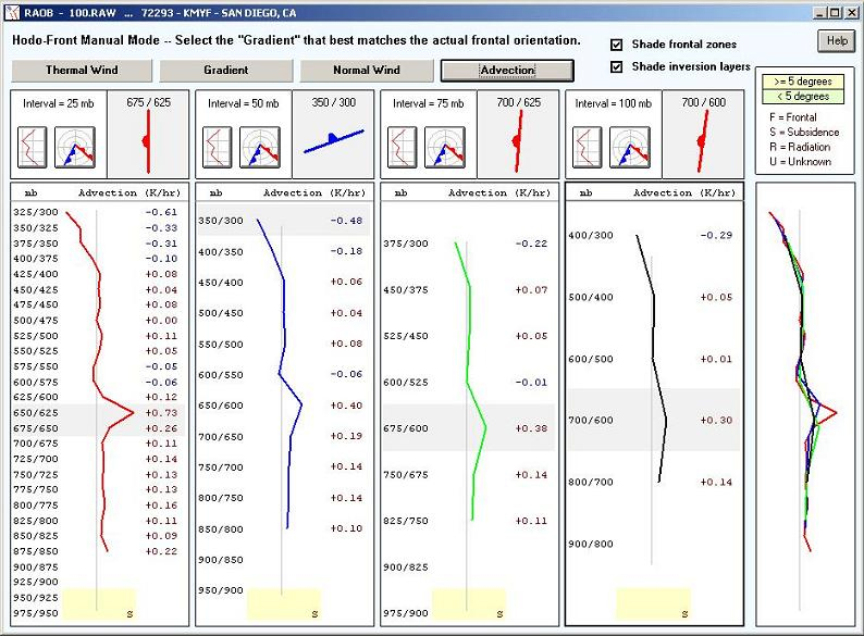
RAOB's Frontal Analysis screen analyses the sounding's winds, generating thermal wind vectors, and then applies the user's configuration parameters to locate the sounding's most significant frontal layers. The selected front is drawn over the hodograph, while key frontal data is listed below the diagram. Even greater detail of the sounding's frontal layers are available by viewing the manual analysis screen. The sounding's thermal winds can also be used create reliable short-term forecasts when no other data is available. See the optional Fronts & Forecast module for more details.
Example Vertical Cross-Section screen

Example of a cross-section screen
This is a distance-based cross-section showing temperature contour analyses of a dataset containing 5 soundings. RAOB can plot up to 100 soundings per cross-section, analyze dozens of significant data parameters in any combination. Parameter intervals, colors, and line types can be individually configured. Using the Standard vertical Cross-Section diagrams, RAOB can generate interpolated soundings from any x-axis location. RAOB can also generate time-based cross-section for time-series analyses. Cross-section diagrams can be completely scaled and configured just like the sounding diagrams.
Example Mountain (lee) Wave screen
 Wave screen")
Example of a Mountain (lee) Wave screen
The Mountain-Wave screen is unique to the RAOB program. This example displays the “predominate” wave produced by a single sounding as associated with specific mountain parameters. At the left side of the diagram are the "original" sounding winds and the “normal” winds (perpendicular to the mountain ridge). At the top are details regarding the mountain's features and resulting wave characteristics A scroll bar at the bottom allows detailed display of the wave’s vertical velocities at any downwind range. For more information, see the Turbulence & Mountain Wave module.